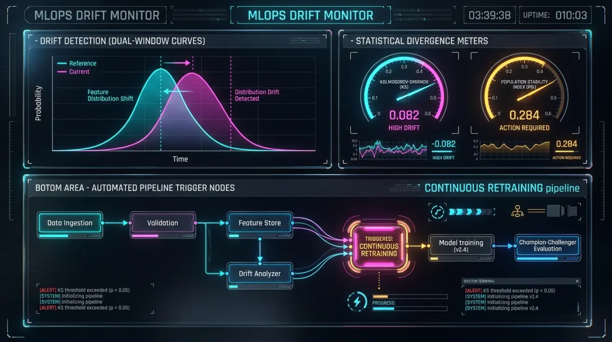
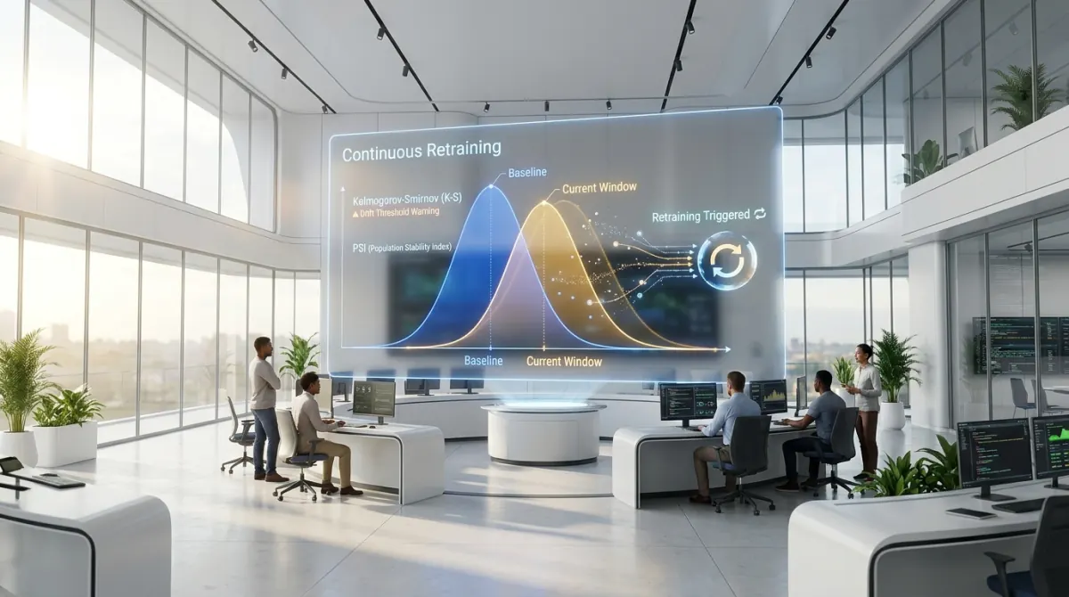
Continuous Retraining Pipelines: Detecting & Handling Conce…

“We publish our benchmarks, failure logs, and cost-per-run data for every system we ship — so you can evaluate results, not promises.” — FalconicLab

A machine learning model begins decaying the exact second it is deployed to production.

In textbook data science, training datasets and inference queries are assumed to be independent and identically distributed ( $\text{i.i.d.}$ ). In live enterprise production—across Banking & Financial Services fraud detection, Retail & E-commerce recommendation engines, and Healthcare & Life Sciences clinical risk triage—the physical world is constantly mutating. Consumer spending habits shift during macroeconomic shocks, adversarial fraud syndicates alter their card-testing patterns, medical reimbursement coding rules change, and seasonal trends invalidate historical baseline distributions.

Most engineering organizations manage this reality with two flawed extremes:

The “Train Once, Pray Forever” Blind Spot: A model is shipped to production and left unmonitored until business stakeholders notice revenue dropping or customer support complaints surging weeks later.
The Uncalibrated Retraining Hamster Wheel: Every minor statistical jitter in an input feature triggers a full automated retraining pipeline in Apache Airflow or Kubeflow. This burns tens of thousands of dollars in redundant GPU training compute, introduces unnecessary deployment instability, and frequently trains models on transient holiday anomalies that degrade long-term performance.

At FalconicLab, our autonomous intelligence platform (PRIMARY_CORE // AUTONOMOUS_V2) operates across mission-critical sectors where performance degradation is unacceptable—including our Sub-50ms Financial Fraud Engine (exp-02, 99.6% precision) and our Intelligent Document Processing Engine (exp-03, 97.8% precision). We maintain model precision over multi-year operational horizons by deploying Continuous Retraining Pipelines grounded in rigorous statistical divergence metrics, automated data validation, and zero-downtime canary shadow deployments.

This deep dive walks technical executives and MLOps platform engineers through the mathematical theory of drift, non-parametric hypothesis testing, population stability indices, automated pipeline orchestration using Airflow and Kubeflow, and a complete, runnable Python continuous drift-detection engine.

Executive Summary: Covariate Shift vs. Concept Drift vs. Prior Shift

For CTOs, Chief Data Officers, and ML Engineering Directors, designing an effective continuous retraining architecture requires establishing a clear mathematical taxonomy of drift. In a supervised machine learning system predicting target variable $Y$ from input features $X$ , the joint probability distribution factors as:

P(X, Y) = P(Y \mid X) \cdot P(X)

A change in this joint distribution over time $t$ can occur in three fundamentally distinct ways:

Drift Category	Formal Mathematical Formulation	Real-World Enterprise Example	Retraining Trigger Decision
Data Drift (Covariate Shift)	$P_t(X) \neq P_0(X)$ , but $P_t(Y \mid X) = P_0(Y \mid X)$	A marketing campaign brings younger users; spending features shift, but relationship to fraud stays constant	Conditional: Do NOT retrain immediately unless confidence margins degrade
Concept Drift (Posterior Shift)	$P_t(Y \mid X) \neq P_0(Y \mid X)$ , while $P(X)$ may remain constant	A new fraud syndicate bypasses OTP checks; previously benign transaction features now represent fraudulent attacks	Mandatory & Urgent: Trigger automated model fine-tuning or structural retraining
Prior Probability Shift	$P_t(Y) \neq P_0(Y)$ , while $P_t(X \mid Y) = P_0(X \mid Y)$	Macroeconomic recession increases baseline loan default rates across all credit score bands	Threshold Recalibration: Recalibrate decision boundaries before executing expensive re-training
Feature / Schema Corruption	Upstream API schema drift, missing columns, or timestamp formatting errors	A third-party payment gateway starts passing `null` for `zip_code` or changes currency encoding	Emergency Circuit Break: Halt inference; do NOT retrain on corrupted inputs!

Continuous retraining and drift control pipeline

Mathematical Foundations of Statistical Drift Detection

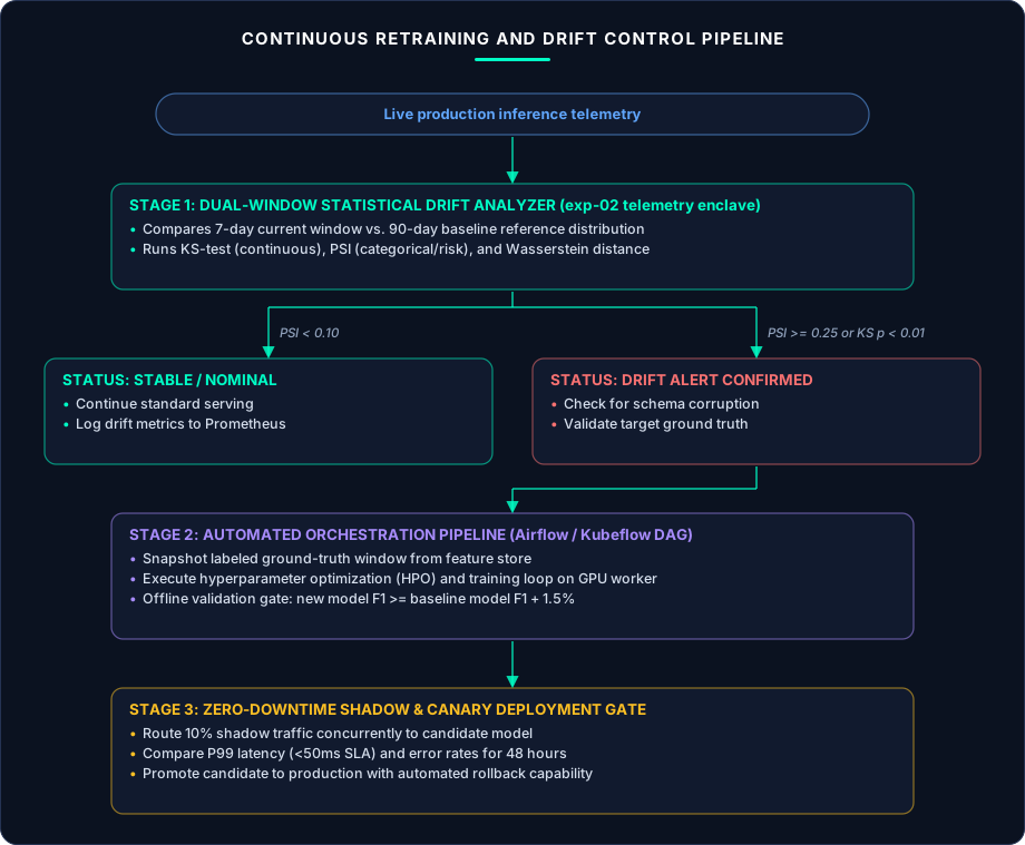
To build an automated system that alerts on genuine concept drift without crying wolf on everyday variance, we employ four complementary statistical tests across our MLOps pipelines on FalconicLab Skills:

1. Kolmogorov-Smirnov (KS) Two-Sample Test (Continuous Features)

The two-sample Kolmogorov-Smirnov test is a non-parametric test evaluating whether two continuous empirical distributions $F_1(x)$ (the 90-day baseline) and $F_2(x)$ (the 7-day production window) were drawn from the same underlying population.

The test statistic $D$ represents the maximum vertical distance between the two cumulative distribution functions (CDFs):

D = \sup_{x} |F_1(x) - F_2(x)|

The null hypothesis $H_0: F_1 = F_2$ is rejected at significance level $\alpha$ (typically $\alpha = 0.01$ ) when:

D > c(\alpha) \sqrt{\frac{n_1 + n_2}{n_1 n_2}}

Where $c(0.01) \approx 1.63$ . If $p\text{-value} < 0.01$ , the feature has drifted with 99% statistical confidence.

2. Population Stability Index (PSI) (Categorical & Binned Features)

Originally developed in commercial banking credit risk models, the Population Stability Index (PSI) measures the overall shift between a reference population $B$ and an evaluation population $T$ across $K$ binned buckets:

\text{PSI} = \sum_{k=1}^{K} \left( \% T_k - \% B_k \right) \times \ln\left( \frac{\% T_k}{\% B_k} \right)

Where:

$\% B_k$ is the proportion of observations in bucket $k$ in the baseline reference dataset.
$\% T_k$ is the proportion of observations in bucket $k$ in the current production dataset.

Standard Enterprise Interpretation Rules

$\text{PSI} < 0.10$ : No Significant Shift. The distribution is stable; no action required.
$0.10 \le \text{PSI} < 0.25$ : Moderate Shift. Requires investigation and monitoring; schedule validation.
$\text{PSI} \ge 0.25$ : Significant Shift. Substantial drift detected; triggers automated retraining pipeline.

3. Wasserstein Distance (Earth Mover’s Distance)

While the KS-test only measures the single point of maximum divergence, the Wasserstein Metric ( $W_1$ ) measures the total geometric work required to transform distribution $u$ into distribution $v$ :

W_1(u, v) = \int_{-\infty}^{\infty} |U(x) - V(x)| \, dx

Where $U(x)$ and $V(x)$ are the respective continuous cumulative distributions. In production financial pipelines, Wasserstein distance is particularly robust because it scales linearly with the magnitude of financial shifts (e.g., transaction amounts shifting by $50 vs. $5,000), unlike $p$ -values which become hyper-sensitive on large sample sizes.

Architectural Pillar: Ground-Truth Latency & The Verification Problem

The hardest operational challenge in continuous retraining is Ground-Truth Label Latency.

In Search Click-Through Rate (CTR) models, ground truth arrives in seconds (the user clicked or did not click).
In Document Extraction (exp-03), ground truth arrives in minutes to hours via Human-in-the-Loop review queues.
In Financial Fraud Detection (exp-02), ground truth is delayed: a fraudulent credit card transaction may not be reported by the cardholder or chargeback network for 30 to 90 days!

How to Trigger Retraining When Labels Are Delayed

If you wait 90 days for fraud labels to arrive before detecting drift, your production model will bleed money for three months. Our MLOps architecture deploys a Two-Tier Monitoring Strategy:

Unsupervised Data Drift Monitoring (Real-Time): Continuously evaluate $P(X)$ daily using KS-tests and PSI across incoming feature vectors. If input features diverge sharply ( $\text{PSI} \ge 0.25$ ) while prediction probability distributions $P(\hat{Y})$ shift simultaneously, flag an Unsupervised Drift Alert.
Supervised Target Verification on Delayed Windows (Bi-Weekly): As confirmed chargebacks and fraud dispute files settle from card networks, compute true precision, recall, and PR-AUC over rolling 30-day cohorts. When true precision drops below the contractual SLA (e.g., $99.6\%$ on exp-02), trigger the automated model retraining DAG.

Production Implementation: Comprehensive Statistical Drift Engine

Below is a complete, runnable Python implementation of our Production Statistical Drift & Automated Retraining Trigger Engine. It implements Kolmogorov-Smirnov continuous testing, 10-bin Population Stability Index (PSI) with epsilon smoothing, Wasserstein distance computation, and automated retraining dispatch criteria.

from __future__ import annotations

import math
from dataclasses import dataclass, field
from enum import Enum
from typing import Any

import numpy as np
from scipy import stats

class DriftSeverity(str, Enum):
    NO_DRIFT = "NO_DRIFT"
    MODERATE_DRIFT = "MODERATE_DRIFT"
    SEVERE_DRIFT_RETRAIN_REQUIRED = "SEVERE_DRIFT_RETRAIN_REQUIRED"

@dataclass
class FeatureDriftReport:
    feature_name: str
    psi_score: float
    ks_statistic: float
    ks_p_value: float
    wasserstein_distance: float
    severity: DriftSeverity
    baseline_sample_size: int
    current_sample_size: int

@dataclass
class PipelineRetrainingVerdict:
    pipeline_id: str
    trigger_retraining: bool
    highest_severity: DriftSeverity
    severe_drift_features: list[str]
    moderate_drift_features: list[str]
    total_features_analyzed: int
    execution_time_ms: float
    detailed_reports: list[FeatureDriftReport] = field(default_factory=list)

class FalconicContinuousDriftEngine:
    """
    FalconicLab Production Statistical Drift & Retraining Decision Engine:
    - Calculates 10-bin Population Stability Index (PSI) with epsilon smoothing
    - Computes Kolmogorov-Smirnov (KS) two-sample test statistics and p-values
    - Evaluates Wasserstein Distance (Earth Mover's Distance)
    - Generates deterministic retraining triggers based on statistical consensus
    """

    def __init__(
        self,
        psi_severe_threshold: float = 0.25,
        psi_moderate_threshold: float = 0.10,
        ks_p_threshold: float = 0.01,
        min_sample_size: int = 100,
    ) -> None:
        self.psi_severe_threshold = psi_severe_threshold
        self.psi_moderate_threshold = psi_moderate_threshold
        self.ks_p_threshold = ks_p_threshold
        self.min_sample_size = min_sample_size

    @staticmethod
    def calculate_psi(
        baseline: np.ndarray,
        current: np.ndarray,
        num_buckets: int = 10,
        epsilon: float = 1e-4,
    ) -> float:
        """
        Calculates Population Stability Index across quantile buckets with epsilon smoothing.
        """
        # Determine quantile bin edges based strictly on baseline distribution
        quantiles = np.linspace(0, 100, num_buckets + 1)
        bin_edges = np.percentile(baseline, quantiles)
        bin_edges[0] = -np.inf
        bin_edges[-1] = np.inf

        # Handle edge case of low-variance constant features
        bin_edges = np.unique(bin_edges)
        if len(bin_edges) <= 2:
            return 0.0

        # Compute counts in each bucket
        baseline_counts, _ = np.histogram(baseline, bins=bin_edges)
        current_counts, _ = np.histogram(current, bins=bin_edges)

        # Convert to relative proportions with epsilon smoothing to prevent div by zero
        baseline_pct = (baseline_counts / len(baseline)) + epsilon
        current_pct = (current_counts / len(current)) + epsilon

        # Normalize proportions so sum equals 1.0
        baseline_pct /= np.sum(baseline_pct)
        current_pct /= np.sum(current_pct)

        # Calculate PSI = sum((Current - Baseline) * ln(Current / Baseline))
        psi_val = np.sum((current_pct - baseline_pct) * np.log(current_pct / baseline_pct))
        return float(round(psi_val, 5))

    def evaluate_feature_drift(
        self,
        feature_name: str,
        baseline_data: np.ndarray,
        current_data: np.ndarray,
    ) -> FeatureDriftReport:
        if len(baseline_data) < self.min_sample_size or len(current_data) < self.min_sample_size:
            raise ValueError(
                f"Sample size below threshold ({self.min_sample_size}) for feature {feature_name}"
            )

        # 1. Population Stability Index
        psi_score = self.calculate_psi(baseline_data, current_data)

        # 2. Kolmogorov-Smirnov Two-Sample Test
        ks_res = stats.ks_2samp(baseline_data, current_data)
        ks_stat = float(round(ks_res.statistic, 5))
        ks_p = float(round(ks_res.pvalue, 6))

        # 3. Wasserstein Distance
        w_dist = float(round(stats.wasserstein_distance(baseline_data, current_data), 5))

        # Determine Severity Level
        if psi_score >= self.psi_severe_threshold and ks_p < self.ks_p_threshold:
            severity = DriftSeverity.SEVERE_DRIFT_RETRAIN_REQUIRED
        elif psi_score >= self.psi_moderate_threshold or ks_p < self.ks_p_threshold:
            severity = DriftSeverity.MODERATE_DRIFT
        else:
            severity = DriftSeverity.NO_DRIFT

        return FeatureDriftReport(
            feature_name=feature_name,
            psi_score=psi_score,
            ks_statistic=ks_stat,
            ks_p_value=ks_p,
            wasserstein_distance=w_dist,
            severity=severity,
            baseline_sample_size=len(baseline_data),
            current_sample_size=len(current_data),
        )

    def evaluate_pipeline_drift(
        self,
        pipeline_id: str,
        baseline_feature_matrix: dict[str, np.ndarray],
        current_feature_matrix: dict[str, np.ndarray],
        max_tolerable_severe_features: int = 1,
    ) -> PipelineRetrainingVerdict:
        import time
        t0 = time.perf_counter()

        reports: list[FeatureDriftReport] = []
        severe_feats: list[str] = []
        moderate_feats: list[str] = []

        for feat_name, base_vec in baseline_feature_matrix.items():
            if feat_name not in current_feature_matrix:
                continue
            curr_vec = current_feature_matrix[feat_name]
            report = self.evaluate_feature_drift(feat_name, base_vec, curr_vec)
            reports.append(report)

            if report.severity == DriftSeverity.SEVERE_DRIFT_RETRAIN_REQUIRED:
                severe_feats.append(feat_name)
            elif report.severity == DriftSeverity.MODERATE_DRIFT:
                moderate_feats.append(feat_name)

        elapsed_ms = round((time.perf_counter() - t0) * 1000.0, 2)

        # Retraining Decision Logic
        should_retrain = len(severe_feats) >= max_tolerable_severe_features
        highest_severity = (
            DriftSeverity.SEVERE_DRIFT_RETRAIN_REQUIRED
            if severe_feats
            else (DriftSeverity.MODERATE_DRIFT if moderate_feats else DriftSeverity.NO_DRIFT)
        )

        return PipelineRetrainingVerdict(
            pipeline_id=pipeline_id,
            trigger_retraining=should_retrain,
            highest_severity=highest_severity,
            severe_drift_features=severe_feats,
            moderate_drift_features=moderate_feats,
            total_features_analyzed=len(reports),
            execution_time_ms=elapsed_ms,
            detailed_reports=reports,
        )

Real Production Failure Logs: Lessons from Continuous Retraining Pipelines

In accordance with FalconicLab’s engineering transparency, below are two real production failure incidents from our automated retraining systems that shaped our current deployment gates.

Failure Log #01: The “Black Friday” Seasonality Retraining Loop

[FALCONIC_MLOPS_TELEMETRY // INCIDENT_LOG_2025_11_29]
pipeline_id: "retraining_worker_dag_retail_ecom_04"
status: "RUNAWAY_RETRAINING_LOOP_DETECTED"
runs_triggered_in_24h: 8
gpu_compute_wasted_usd: $4,280.00
root_cause: "HOLIDAY_PURCHASE_VOLUME_SPIKE_MISCLASSIFIED_AS_PERMANENT_DRIFT"

What Happened: On Black Friday, transaction volume and cart sizes increased by 450% across an e-commerce platform in Retail & E-commerce. The automated monitoring daemon detected a massive feature shift on cart_total_usd ( $\text{PSI} = 0.52$ ) and automatically triggered an Airflow retraining job. The new model trained on Black Friday surge data over-indexed on extreme purchase amounts. Forty-eight hours later, when shopping volume returned to baseline, the new model flagged standard purchases as anomalies, triggering another retraining run!
The Architectural Fix:
1. Calendar & Seasonality Exclusion Mask: Added deterministic holiday calendar masks to the drift detection daemon. During known peak retail windows (Black Friday, Cyber Monday, Prime Day), automated retraining triggers are locked to prevent training on transient distribution spikes.
2. Multi-Window Consensus Requirement: A feature must exhibit sustained severe drift across three consecutive 24-hour evaluation windows before an automated retraining pipeline is permitted to execute.

Failure Log #02: Upstream Sensor Calibration Drift in Smart Manufacturing

[FALCONIC_MLOPS_TELEMETRY // INCIDENT_LOG_2026_04_08]
pipeline_id: "industrial_iot_bearing_fault_scorer"
sector: "Manufacturing & Smart Industry"
symptom: "Model False Positive Rate surged from 0.4% to 14.8%"
root_cause: "HARDWARE_SENSOR_RECALIBRATION_CHANGED_UNIT_SCALE_WITHOUT_FEATURE_STORE_UPDATE"

What Happened: In a predictive maintenance deployment in Manufacturing & Smart Industry, a physical vibration sensor on a turbine was replaced during scheduled maintenance. The new sensor reported acceleration in $\text{m/s}^2$ instead of imperial $g$ -force ( $1g \approx 9.81 \, \text{m/s}^2$ ). Because the pipeline lacked an automated feature-store contract validator, the model ingested numbers roughly 10x larger than normal.
The Architectural Fix: Before running statistical drift tests or retraining DAGs, all incoming data must pass Great Expectations / Pydantic Data Contract Gates verifying min/max ranges, null fractions, and unit dimensions. Sensor unit scaling errors are now blocked at data ingestion in under 2ms.

Zero-Downtime Deployment: The Shadow & Canary Verification Architecture

When an automated retraining pipeline successfully compiles and trains a new model candidate $M_{\text{new}}$ , never deploy it directly to live user traffic.

At FalconicLab, all retrained models pass through a 48-Hour Shadow Deployment Funnel:

Zero-downtime canary and shadow deployment funnel

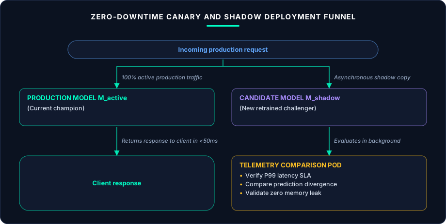
Shadow Traffic Mirrored: The API gateway routes 100% of live traffic to the current champion model $M_{\text{active}}$ while asynchronously broadcasting a shadow copy to $M_{\text{shadow}}$ .
Side-by-Side Telemetry Comparison: For 48 hours, an observability pod computes latency distributions (verifying the sub-50ms SLA), prediction divergence, and system memory consumption without impacting live customers.
Canary Promotion: If $M_{\text{shadow}}$ matches latency SLAs and demonstrates superior accuracy on emerging ground truth, the gateway shifts live traffic in increments: $5\% \rightarrow 25\% \rightarrow 100\%$ , with an automated rollback trigger if error rates spike.

6 Engineering Rules for Continuous Retraining

Distinguish Covariate Shift from True Concept Drift: Never trigger costly GPU training solely because an input feature shifted. Verify whether prediction confidence margins or true performance metrics are actually degrading.
Enforce Dual-Window Hypothesis Testing: Compare short-term production windows (7 days) against robust long-term baselines (90 days) using both non-parametric KS-tests and 10-bin Population Stability Index (PSI).
Apply Seasonality & Holiday Exclusion Masks: Lock automated training pipelines during known calendar spikes (Black Friday, tax deadlines, holidays) to prevent models from over-fitting on temporary behavioral spikes.
Require Multi-Window Consensus: A feature must exhibit sustained severe drift across at least three consecutive daily evaluation cycles before an automated retraining pipeline is initiated.
Enforce Pre-Training Data Contract Validation: Verify schema integrity, min/max bounds, and null percentages using deterministic data contract validators to prevent retraining on corrupted sensor streams.
Always Verify Candidate Models in Shadow Mode: Run retrained models in zero-downtime shadow mode for 48 hours against live mirrored traffic before initiating progressive canary rollouts.

Build Robust Production ML Pipelines With FalconicLab

Prevent silent model degradation and eliminate wasteful retraining loops with production-grade MLOps architecture. Explore our high-precision machine learning nodes on FalconicLab Experiments, review our engineering capabilities across FalconicLab Skills, or consult with our MLOps systems architects via FalconicLab Contact.